Predict Method for Linear Model Fits

The function predict.lm in EnvStats is a modified version of the built-in R function predict.lm. The only modification is that for the EnvStats function predict.lm, if se.fit=TRUE, the list returned includes a component called n.coefs. The component n.coefs is used by the function pointwise to create simultaneous confidence or prediction limits.

# S3 method for class 'lm'
predict(object, ...)

Arguments

object: Object of class inheriting from "lm".
...: Further arguments passed to the R function predict.lm. See the R help file for the R function predict.lm.

Details

See the R help file for predict.lm.

Value

See the R help file for predict.lm.

The only modification is that for the EnvStats function predict.lm, if se.fit=TRUE, the list returned includes a component called n.coefs, i.e., the function returns a list with the following components:

fit: vector or matrix as above
se.fit: standard error of predicted means
residual.scale: residual standard deviations
df: degrees of freedom for residual
n.coefs: numeric scalar denoting the number of predictor variables used in the model

References

Chambers, J.M., and Hastie, T.J., eds. (1992). Statistical Models in S. Chapman and Hall/CRC, Boca Raton, FL.

Draper, N., and H. Smith. (1998). Applied Regression Analysis. Third Edition. John Wiley and Sons, New York, Chapter 3.

Millard, S.P., and N.K. Neerchal. (2001). Environmental Statistics with S-PLUS. CRC Press, Boca Raton, FL, pp.546-553.

Miller, R.G. (1981a). Simultaneous Statistical Inference. Springer-Verlag, New York, pp.111, 124.

Author

R Development Core Team (for code for R version of predict.lm).

Steven P. Millard (for modification to add compenent n.coefs; EnvStats@ProbStatInfo.com)

Examples

  # Using the data from the built-in data frame Air.df, 
  # fit the cube-root of ozone as a function of temperature, 
  # then compute predicted values for ozone at 70 and 90 degrees F,
  # along with the standard errors of these predicted values.

  # First look at the data
  #-----------------------
  with(Air.df, 
    plot(temperature, ozone, xlab = "Temperature (degrees F)", 
      ylab = "Cube-Root Ozone (ppb)"))


  # Now create the lm object 
  #-------------------------
  ozone.fit <- lm(ozone ~ temperature, data = Air.df) 


  # Now get predicted values and CIs at 70 and 90 degrees.
  # Note the presence of the last component called n.coefs.
  #--------------------------------------------------------
  predict.list <- predict(ozone.fit, 
    newdata = data.frame(temperature = c(70, 90)), se.fit = TRUE) 

  predict.list
#> $fit
#>        1        2 
#> 2.697810 4.101808 
#> 
#> $se.fit
#>          1          2 
#> 0.07134554 0.08921071 
#> 
#> $df
#> [1] 114
#> 
#> $residual.scale
#> [1] 0.5903046
#> 
#> $n.coefs
#> [1] 2
#> 
  #$fit
  #       1        2 
  #2.697810 4.101808 
  #
  #$se.fit
  #         1          2 
  #0.07134554 0.08921071 
  #
  #$df
  #[1] 114
  #
  #$residual.scale
  #[1] 0.5903046
  #
  #$n.coefs
  #[1] 2

 
  #----------

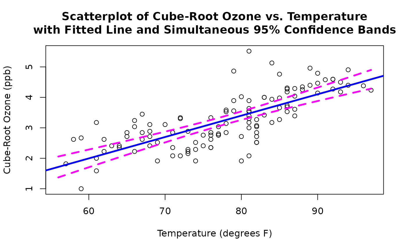
  #Continuing with the above example, create a scatterplot of 
  # cube-root ozone vs. temperature, and add the fitted line 
  # along with simultaneous 95% confidence bands.

  with(Air.df, 
    plot(temperature, ozone, xlab = "Temperature (degrees F)", 
      ylab = "Cube-Root Ozone (ppb)"))

  abline(ozone.fit, lwd = 3, col = "blue")

  new.temp <- with(Air.df, 
    seq(min(temperature), max(temperature), length = 100))

  predict.list <- predict(ozone.fit, 
    newdata = data.frame(temperature = new.temp), 
    se.fit = TRUE)

  ci.ozone <- pointwise(predict.list, coverage = 0.95, 
    simultaneous = TRUE)

  lines(new.temp, ci.ozone$lower, lty = 2, lwd = 3, col = "magenta") 

  lines(new.temp, ci.ozone$upper, lty = 2, lwd = 3, col = "magenta") 

  title(main=paste("Scatterplot of Cube-Root Ozone vs. Temperature", 
    "with Fitted Line and Simultaneous 95% Confidence Bands", 
    sep="\n"))


  #----------

  # Clean up
  #---------
  rm(ozone.fit, predict.list, new.temp, ci.ozone)
  graphics.off()